Posterior sampling (MCMC)

Instead—or on top—of running the Profiler to obtain credible intervals for the parameter estimates, we can also run an MCMC sampler to generate a proper posterior sample. This allows estimating the actual marginal distributions for each parameter.

This tutorial provides an exemplatory implementation of an MCMC sampler for posterior sampling. We use the sampler implementation provided by noctiluca; of course you can adapt this to use your favorite MCMC implementation.

from copy import deepcopy
import numpy as np
from matplotlib import pyplot as plt
from scipy import stats

from noctiluca.util import mcmc
import bayesmsd

Set up

We generate an example dataset with 100 trajectories à 20 frames, with \(\text{MSD}(\Delta t) = \sqrt{\Delta t}\) and fit it with a powerlaw MSD, hoping to recover the parameters \(\Gamma = 1\) and \(\alpha = 0.5\).

np.random.seed(186875736)
data = bayesmsd.gp.generate((bayesmsd.deco.MSDfun(lambda dt: np.sqrt(dt)), 1, 1), T=100, n=20)

fit = bayesmsd.lib.NPXFit(data, ss_order=1)
fit.parameters['log(σ²) (dim 0)'].fix_to = -np.inf
fitres = fit.run(show_progress=True)

# Print results
for name, val in fitres['params'].items():
    print(f"{name:>15s} = {val:.5f}")

 log(Γ) (dim 0) = 0.01682
      α (dim 0) = 0.48489
log(σ²) (dim 0) = -inf

For reference, let us also run the Profiler. This is just so that we can include the found credible intervals in the plots at the end; otherwise this will be ignored for the rest of the tutorial.

profiler = bayesmsd.Profiler(fit)
profiler.point_estimate = fitres
mci = profiler.find_MCI(show_progress=True)

Writing an MCMC sampler

As mentioned above, we rely on the base MCMC implementation provided by noctiluca. For basic usage, refer to its reference page.

Class definition and constructor

class PosteriorSampler(mcmc.Sampler):
    def __init__(self, fit, fitresult, stepsizes):
        """
        stepsizes: {name : stepsize for name in <(independent) parameters>}
        """
        self.fit = fit
        if fitresult is None:
            self.initial_params = fit.initial_params()
        else:
            self.initial_params = fitresult['params']
        self.stepsizes = stepsizes

        self.min_target_from_fit = self.fit.MinTarget(self.fit)
        self.independent_parameters = self.min_target_from_fit.param_names
...

We initialize the sampler from a Fit instance, which holds the data and defines the posterior (likelihood * prior) that we wish to sample. For the most part it makes sense to actually run the fit and then use the MCMC to sample the posterior around the found point estimate. However, you can of course also skip the fit altogether and just start the MCMC from some initial parameter guess; incidentally, Fit provides such an initial estimate as well.

Implementing the MCMC scheme

The mcmc.Sampler base class takes care of running the MCMC, once we define the basic scheme. This is done by overriding the methods logL() (which defines the likelihood function) and propose_update() (which defines the proposal steps).

...
    def logL(self, params):
        params_array = self.min_target_from_fit.params_dict2array(params)
        return -self.min_target_from_fit(params_array)
...

This one is pretty straight-forward: the min_target_from_fit is essentially the likelihood function (up to a sign, because the fit minimizes). So let’s move on to the proposal step:

...
    def propose_update(self, current_params):
        name = np.random.choice(self.independent_parameters)
        new_params = deepcopy(current_params)
        step_dist = stats.norm(scale=self.stepsizes[name])
        step = step_dist.rvs()
        new_params[name] += step

        return new_params, step_dist.logpdf(step), step_dist.logpdf(-step)
...

This is also not very complicated: we randomly pick a parameter to update and then take a normally distributed step. One could also perform a multivariate update step here (i.e. pick all parameters anew).

The propose_update() method should always return the new parameters and the forward/backward probabilities; the latter are necessary to ensure that the MCMC converges to the correct limiting distribution. Note, however, how in this example the two values will always be identical, since the Gaussian proposal distribution step_dist is symmetric. In that case we could also omit the evaluation of the distribution altogether and just return new_params, 1, 1.

Additional functionality

To make the code from this example directly useable for real applications, we add some convenience.

One great way to use the MCMC sampler is to first run the profiler to get an idea for the width of the posterior in parameter space, and only then move on to the MCMC to get an estimate of the actual marginals. This has the advantage that we can skip the burn-in period of the MCMC sampler, making the procedure one bit less dependent on heuristics. To facilitate this workflow, use the below for initalization from a Profiler and its results (mci):

...
    @classmethod
    def fromProfiler(cls, profiler, mci):
        stepsizes = {name : np.min(np.abs(ci - m)) for name, (m, ci) in mci.items()}
        return cls(profiler.fit,
                   profiler.point_estimate,
                   stepsizes,
                  )
...

Finally, the run() method of mcmc.Sampler usually expects initial values from the user. But we know good starting points, so for convenience we override as follows:

...
    def run(self):
        return super().run(self.initial_params)

Full implementation

In summary, we obtain the following implementation of the PosteriorSampler:

class PosteriorSampler(mcmc.Sampler):
    def __init__(self, fit, fitresult, stepsizes):
        """
        stepsizes: {name : stepsize for name in <(independent) parameters>}
        """
        self.fit = fit
        if fitresult is None:
            self.initial_params = fit.initial_params()
        else:
            self.initial_params = fitresult['params']
        self.stepsizes = stepsizes

        self.min_target_from_fit = self.fit.MinTarget(self.fit)
        self.independent_parameters = self.min_target_from_fit.param_names

    @classmethod
    def fromProfiler(cls, profiler, mci):
        stepsizes = {name : np.min(np.abs(ci - m)) for name, (m, ci) in mci.items()}
        return cls(profiler.fit,
                   profiler.point_estimate,
                   stepsizes,
                  )

    def logL(self, params):
        params_array = self.min_target_from_fit.params_dict2array(params)
        return -self.min_target_from_fit(params_array)

    def propose_update(self, current_params):
        name = np.random.choice(self.independent_parameters)
        new_params = deepcopy(current_params)
        step_dist = stats.norm(scale=self.stepsizes[name])
        step = step_dist.rvs()
        new_params[name] += step

        return new_params, step_dist.logpdf(step), step_dist.logpdf(-step)

    def run(self):
        return super().run(self.initial_params)

Running the sampler

The posterior sampler can now be used through the interface provided by mcmc.Sampler. The unfamiliar reader can consult the relevant documentation; but for the most part the usage is straight-forward: we initialize the PosteriorSampler, configure it to our liking and finally let it run.

Note that here we initialize the MCMC just from the fit we ran above and guess* good step sizes for the two free parameters. Alternatively we could initialize the stepsizes from the measured credible intervals; for this example, however, let’s keep MCMC and Profiler independent, such that we can show a fair comparison below.

(*) by “guess” we mean that these are chosen such that the acceptance rate of the sampler is about 50%.

sampler = PosteriorSampler(fit, fitres, stepsizes={'log(Γ) (dim 0)' : 0.05, 'α (dim 0)' : 0.05})
sampler.configure(iterations = 1000,
                  burn_in = 100,
                  log_every = 100,
                  show_progress=True,
                 )
mcmcrun = sampler.run()

iteration 100: acceptance = 50%, logL = -2684.452983934565
iteration 200: acceptance = 50%, logL = -2683.8686291046965
iteration 300: acceptance = 52%, logL = -2685.1974716015793
iteration 400: acceptance = 49%, logL = -2684.239537156863
iteration 500: acceptance = 49%, logL = -2687.1646074106
iteration 600: acceptance = 49%, logL = -2685.190189087895
iteration 700: acceptance = 50%, logL = -2683.8508050453365
iteration 800: acceptance = 50%, logL = -2684.6226215158495
iteration 900: acceptance = 50%, logL = -2684.4366339655567
iteration 1000: acceptance = 51%, logL = -2683.7854148854503

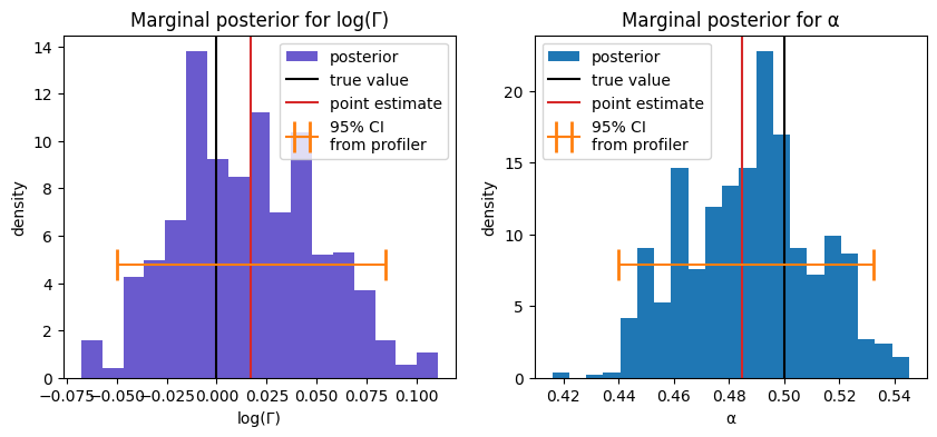
# Plot results
fig, axs = plt.subplots(1, 2, figsize=[10, 4])

for (ax,
     name,
     color,
     true_value,
    ) in zip(axs,
             ['log(Γ)', 'α'],
             ['slateblue', 'tab:blue'],
             [0, 0.5],
            ):

    samples = np.array([params[name+' (dim 0)'] for params in mcmcrun.samples])
    ax.hist(samples, bins='auto', density=True, color=color, label='posterior')

    ax.axvline(true_value, color='k', label='true value')

    m, ci = mci[name+' (dim 0)']
    ax.axvline(m, color='tab:red', label='point estimate')

    ax.set_ylim([0, None])
    _, ytop = ax.get_ylim()
    yci = 0.33*ytop
    ax.errorbar(m, yci, xerr=np.abs(ci-m)[:, None],
                color='tab:orange', label='95% CI\nfrom profiler',
                capsize=10, capthick=2,
                zorder=3,
               )

    ax.legend()
    ax.set_xlabel(name)
    ax.set_ylabel('density')
    ax.set_title('Marginal posterior for '+name)

plt.show()