Likelihood landscapes
bayesmsd being a Bayesian framework means that its central object is the likelihood function, i.e. the function that—based on the input data—assigns statistical weights to all parameter combinations.
The bayesmsd package is predominantly focussed on defining, computing, and optimizing this function, i.e. the practical needs for application. For debugging or learning, however, it can also be very instructive to visualize the whole likelihood landscape, instead of blindly trusting the code to find its way through it; this will be the subject of the present example.
[1]:
import os
os.environ['OMP_NUM_THREADS'] = '1'

from tqdm.auto import tqdm
import itertools
import numpy as np
from matplotlib import pyplot as plt

import noctiluca as nl
import bayesmsd
We start by generating a simple, subdiffusive data set with \(\text{MSD} = \sqrt{\Delta t} \equiv \Gamma\left(\Delta t\right)^\alpha\) with \(\Gamma = 1\) and \(\alpha = 0.5\). We fit a powerlaw (no localization error) to these data:
[2]:
np.random.seed(84567719)
data = bayesmsd.gp.generate((bayesmsd.deco.MSDfun(lambda dt: dt**0.5), 1, 1), T=100, n=20)

fit = bayesmsd.lib.NPXFit(data, ss_order=1)
fit.parameters['log(σ²) (dim 0)'].fix_to = -np.inf
fitres = fit.run(show_progress=True)

for name, val in fitres['params'].items():
    print(f"{name:>15s} = {val:.5f}")
 log(Γ) (dim 0) = 0.02426
      α (dim 0) = 0.48947
     m1 (dim 0) = 0.00000
log(σ²) (dim 0) = -inf
The results look decent, though not perfect; this is expected, because our data set contains relatively little data (20 trajectories à 100 frames each). This means that we expect a broad peak in the likelihood landscape. Let’s take a look.
We begin by pulling the likelihood function* from the fit object:
[3]:
neg_logL = fit.MinTarget(fit)
def log_likelihood(params):
    return -neg_logL(neg_logL.params_dict2array(params))
What’s happening here? The core objective of the fit is to find parameter values that maximize the likelihood function. Technically, it does so by minimizing the negative (log-)likelihood; we can thus grab the (log-)likelihood function from the internal “minimization target”. The returned object expects parameter values as a simple numpy array (as required by scipy.optimize.minimize); so we construct a little wrapper taking care of the conversion from the more verbose dict structure that
e.g. fitres['params'] employs.
This gives us the function log_likelihood(), which takes parameters in the same format as fitres['params'] and gives the corresponding (log-)likelihood values.
*technically, this is the unnormalized posterior, i.e. it contains the priors applied by bayesmsd; it is just not normalized to be a proper posterior distribution.
What’s left to do now is to evaluate this function on a grid of parameter values and display the resulting landscape:
[4]:
logG, a = np.meshgrid(np.log(np.linspace(0.7, 1.3, 20)), np.linspace(0.3, 0.7, 20))
logL = np.nan*np.empty(logG.shape)

for i, j in itertools.product(*list(map(range, logL.shape))):
    params = {key : val for key, val in fitres['params'].items()} # copy point estimate
    params['log(Γ) (dim 0)'] = logG[i, j] # adjust sweeping
    params[     'α (dim 0)'] =    a[i, j] # parameters

    logL[i, j] = log_likelihood(params)   # evaluate
[5]:
# Plot
h = plt.pcolormesh(np.exp(logG), a, logL-np.max(logL),
                   shading='nearest',
                   vmin=-10,
                  )

plt.scatter(1, 0.5,
            marker='x', color='r',
            label='true parameters',
           )
plt.scatter(np.exp(fitres['params']['log(Γ) (dim 0)']),
            fitres['params']['α (dim 0)'],
            marker='x', color='k',
            label='fitted parameters\n(likelihood maximum)',
           )

plt.legend()
plt.colorbar(h, label='log(L)')
plt.xlabel('Γ')
plt.ylabel('α')
plt.title('Likelihood landscape')

plt.show()
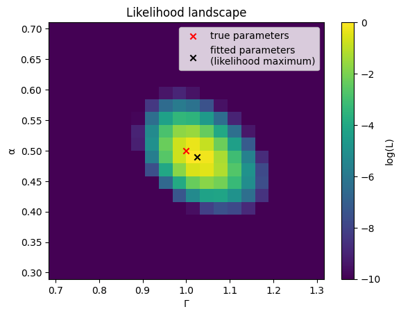
And here we go: a direct illustration of the likelihood landscape underlying the fit.
A note of caution: log-likelihoods have a linear scale
When studying log-likelihood functions/landscapes, we have to think in absolute terms: a difference of one point in the log-likelihood means that the statistical weights of the corresponding parameter sets differ by a factor of \(\mathrm{e}^1 = 2.72\). Differences of more than a few points in log-likelihood should thus be thought of as very strong distinctions.
This point about considering absolute differences is important to keep in mind, especially because the actual values of the log-likelihood function can be enormous in magnitude. They depend on the size of the data set and can easily reach values in the millions and billions. For our relatively small example data set here, this effect is not as drastic, but still notable:
[6]:
print(f"actual likelihood values:")
print(f"  minimum:    {np.min(logL):>8.2f}")
print(f"  maximum:    {np.max(logL):>8.2f}")
print(f"  difference: {np.max(logL)-np.min(logL):>8.2f}")
print(f"  ratio:      {np.max(logL)/np.min(logL):>8.2f}")
actual likelihood values:
  minimum:    -2919.97
  maximum:    -2694.20
  difference:   225.76
  ratio:          0.92
So:
we do not care that the minimum and maximum of the log-likelihood values in our sweep are within 10% of each other
what we do care about is that they are 226 points apart
do not get confused when your maximum log-likelihood evaluates to
-98,165,761; it just means that the plausible parameters are roughly in the range[-98,165,755, -98,165,761].
Higher dimensional parameter space
The example above has a two dimensional parameter space, which is quite convenient for visualization; but usually we have more parameters than that.
In those cases, it often becomes
computationally very expensive to evaluate the likelihood function over a whole grid; this is where the
Profilershinesdifficult to find a good visualization for a function over a multi-dimensional space.
A decent solution for the visualization in a 3D parameter space is a max-projection along the three coordinate axes, which we illustrate here; mostly to provide a reusable code snippet.
We follow the same structure as above, but add in some Gaussian localization error, which will be the third parameter in the fit.
[7]:
np.random.seed(98732457)
true_s = 2
true_G = 1
true_a = 1
data = bayesmsd.gp.generate((bayesmsd.deco.MSDfun(lambda dt: true_G*dt**true_a + 2*true_s**2), 1, 1),
T=100,
n=20,
)
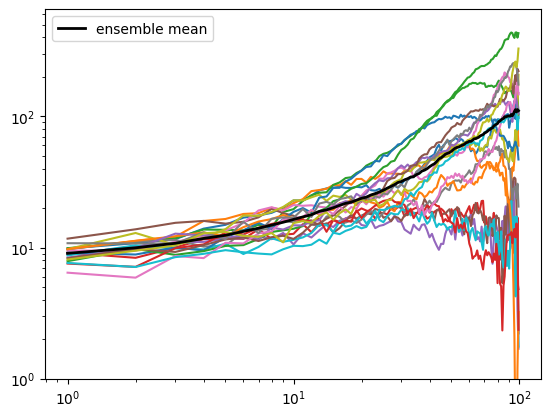
# visualize the empirical MSD before fitting
nl.plot.msd_overview(data)
plt.ylim([1, None])
plt.show()
fit = bayesmsd.lib.NPXFit(data, ss_order=1)
fitres = fit.run(show_progress=True)
for name, val in fitres['params'].items():
print(f"{name:>15s} = {val:.5f}")
log(σ²) (dim 0) = 1.40790
 log(Γ) (dim 0) = -0.11558
      α (dim 0) = 0.97170
     m1 (dim 0) = 0.00000
[8]:
neg_logL = fit.MinTarget(fit)
def log_likelihood(params):
    return -neg_logL(neg_logL.params_dict2array(params))
[9]:
sweep_s = np.linspace(1.7, 2.3, 10)
sweep_G = np.linspace(0.3, 1.7, 10)
sweep_a = np.linspace(0.6, 1.4, 10)
logs2, logG, a = np.meshgrid(2*np.log(sweep_s), np.log(sweep_G), sweep_a,
                             indexing='ij',
                            )
logL = np.nan*np.empty(logG.shape)

for i, j, k in tqdm(itertools.product(*list(map(range, logL.shape)))):
    params = {key : val for key, val in fitres['params'].items()} # copy point estimate
    params['log(σ²) (dim 0)'] = logs2[i, j, k] # adjust
    params[ 'log(Γ) (dim 0)'] =  logG[i, j, k] # sweeping
    params[      'α (dim 0)'] =     a[i, j, k] # parameters

    logL[i, j, k] = log_likelihood(params)   # evaluate
[10]:
fig, axs = plt.subplots(2, 2, figsize=[10, 10],
                        sharex='col', sharey='row',
                        gridspec_kw = {'hspace' : 0.05, 'wspace' : 0.05},
                       )

max_logL = np.max(logL)
vlim = (-10, 0)

ax = axs[1, 1]
h = ax.pcolormesh(sweep_G, sweep_a,
                  np.max((logL-max_logL), axis=0).T,
                  shading='nearest',
                  vmin=vlim[0], vmax=vlim[1],
                 )
ax.scatter(true_G, true_a,
           marker='x', color='r',
          )
ax.scatter(np.exp(fitres['params']['log(Γ) (dim 0)']),
           fitres['params']['α (dim 0)'],
           marker='x', color='k',
          )

ax = axs[1, 0]
ax.pcolormesh(sweep_s, sweep_a,
              np.max(logL-max_logL, axis=1).T,
              shading='nearest',
              vmin=vlim[0], vmax=vlim[1],
             )
ax.scatter(true_s, true_a,
           marker='x', color='r',
          )
ax.scatter(np.exp(0.5*fitres['params']['log(σ²) (dim 0)']),
           fitres['params']['α (dim 0)'],
           marker='x', color='k',
          )

ax = axs[0, 1]
ax.pcolormesh(sweep_G, sweep_s,
              np.max(logL-max_logL, axis=2),
              shading='nearest',
              vmin=vlim[0], vmax=vlim[1],
             )
ax.scatter(true_G, true_s,
           marker='x', color='r',
          )
ax.scatter(np.exp(fitres['params']['log(Γ) (dim 0)']),
           np.exp(0.5*fitres['params']['log(σ²) (dim 0)']),
           marker='x', color='k',
          )

plt.colorbar(h, ax=axs[0, 0],
             label='log-likelihood',
             location='top',
             shrink=0.65,
             fraction=0.7,
            )
axs[0, 0].remove()

ax = axs[0, 1]
ax.scatter(np.nan, np.nan, marker='x', color='r', label='true parameters')
ax.scatter(np.nan, np.nan, marker='x', color='k', label='fit results')
ax.legend(loc=(-0.75, 0.1))

axs[1, 0].set_ylabel('α')
axs[1, 0].set_xlabel('σ')
axs[0, 1].set_ylabel('σ')
axs[0, 1].yaxis.set_tick_params(labelleft=True)
axs[0, 1].invert_yaxis()
axs[1, 1].set_xlabel('Γ')

fig.suptitle('max-projections of likelihood landscape')

plt.show()
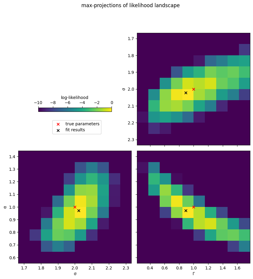
Note how in this example the prefactor \(\Gamma\) has a broad range of likely values. This is because there is a certain tradeoff between the powerlaw and error terms in the MSD: the data given is consistent with MSDs that have a higher exponent, but therefore higher localization error, or, conversely, somewhat lower exponent and therefore also somewhat lower localization error (c.f. bottom left plot).
In practice, results like these simply mean that with the given amount of data we cannot constrain the parameters very precisely: remember that for this example we are studying a data set of 20 trajectories, 100 frames each.
Tips and tricks
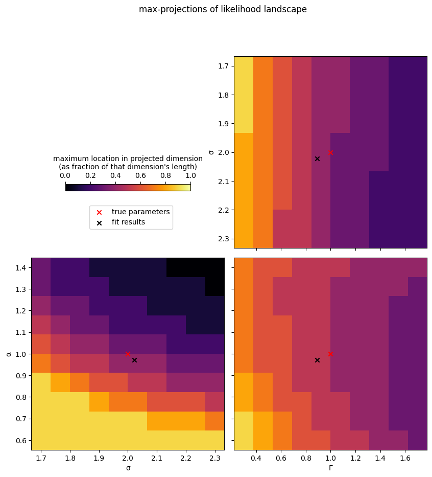
When using the above code snippet to study likelihood landscapes, keep in mind that maximum projections can be tricky to interpret, especially when using large grid spacings (i.e. low resolutions; which one might like to do for computational efficiency). Specifically, one might encounter aliasing effects (such as the apparent non-monotonicity around \(\Gamma\approx 1.2\) in the above example), when the location of the maximum moves from one index in the hidden dimension to the next; it is therefore sometimes useful to
re-run the computation with a finer grid (computationally expensive)
keep in mind that the likelihood function is usually truly pretty smooth (i.e. ignore minor artifacts; can be risky if you are not sure what to take seriously and what not)
in addition to
max(), also look atargmax()maps, i.e. check where in the projected dimension the maximum is located. This can help identify aliasing artifacts.
This last point can be done quite easily by adapting the snippet above (replacing max() by argmax() and changing colormap):
[11]:
fig, axs = plt.subplots(2, 2, figsize=[10, 10],
                        sharex='col', sharey='row',
                        gridspec_kw = {'hspace' : 0.05, 'wspace' : 0.05},
                       )

max_logL = np.max(logL)
vlim = (0, 1)

ax = axs[1, 1]
h = ax.pcolormesh(sweep_G, sweep_a,
                  np.argmax((logL-max_logL), axis=0).T/len(sweep_s),
                  shading='nearest',
                  vmin=vlim[0], vmax=vlim[1],
                  cmap='inferno',
                 )
ax.scatter(true_G, true_a,
           marker='x', color='r',
          )
ax.scatter(np.exp(fitres['params']['log(Γ) (dim 0)']),
           fitres['params']['α (dim 0)'],
           marker='x', color='k',
          )

ax = axs[1, 0]
ax.pcolormesh(sweep_s, sweep_a,
              np.argmax(logL-max_logL, axis=1).T/len(sweep_G),
              shading='nearest',
              vmin=vlim[0], vmax=vlim[1],
              cmap='inferno',
             )
ax.scatter(true_s, true_a,
           marker='x', color='r',
          )
ax.scatter(np.exp(0.5*fitres['params']['log(σ²) (dim 0)']),
           fitres['params']['α (dim 0)'],
           marker='x', color='k',
          )

ax = axs[0, 1]
ax.pcolormesh(sweep_G, sweep_s,
              np.argmax(logL-max_logL, axis=2)/len(sweep_a),
              shading='nearest',
              vmin=vlim[0], vmax=vlim[1],
              cmap='inferno',
             )
ax.scatter(true_G, true_s,
           marker='x', color='r',
          )
ax.scatter(np.exp(fitres['params']['log(Γ) (dim 0)']),
           np.exp(0.5*fitres['params']['log(σ²) (dim 0)']),
           marker='x', color='k',
          )

plt.colorbar(h, ax=axs[0, 0],
             label=('maximum location in projected dimension\n'
                    '(as fraction of that dimension\'s length)'
                   ),
             location='top',
             shrink=0.65,
             fraction=0.7,
            )
axs[0, 0].remove()

ax = axs[0, 1]
ax.scatter(np.nan, np.nan, marker='x', color='r', label='true parameters')
ax.scatter(np.nan, np.nan, marker='x', color='k', label='fit results')
ax.legend(loc=(-0.75, 0.1))

axs[1, 0].set_ylabel('α')
axs[1, 0].set_xlabel('σ')
axs[0, 1].set_ylabel('σ')
axs[0, 1].yaxis.set_tick_params(labelleft=True)
axs[0, 1].invert_yaxis()
axs[1, 1].set_xlabel('Γ')

fig.suptitle('max-projections of likelihood landscape')

plt.show()